In data science, operational efficiency is key to handling increasingly complex and large datasets. GPU acceleration has become essential for modern workflows, offering significant performance improvements.
RAPIDS is a suite of open-source libraries and frameworks developed by NVIDIA, designed to accelerate data science pipelines using GPUs with minimal code changes. Providing tools like cuDF for data manipulation, cuML for machine learning, and cuGraph for graph analytics, RAPIDS enables seamless integration with existing Python libraries, making it easier for data scientists to achieve faster and more efficient processing.
This post shares tips for transitioning from CPU data science libraries to GPU-accelerated workflows, especially for experienced data scientists.
Setting up RAPIDS on desktop or cloud infrastructure
Getting started with RAPIDS is straightforward, but it does have several dependencies. The recommended approach is to follow the official RAPIDS Installation Guide, which provides detailed instructions for local installations. You have multiple paths to install the framework: through pip install, Docker image, or through an environment such as Conda. To set up RAPIDS in a cloud environment, see the RAPIDS Cloud Deployment Guide. Before installing, ensure compatibility by checking your CUDA version and the supported RAPIDS version on the installation page.

cuDF and GPU acceleration for pandas
An advantage of RAPIDS lies in its modular architecture, which empowers users to adopt specific libraries designed for GPU-accelerated workflows. Among these, cuDF stands out as a powerful tool for seamlessly transitioning from traditional pandas-based workflows to GPU-optimized data processing, and requires zero code changes.
To get started, make sure to enable the cuDF extension before importing pandas for execution of data import and remainder of the operation on GPU. By loading the RAPIDS extension with %load_ext cudf.pandas, you can effortlessly integrate cuDF DataFrame within existing workflows, preserving the familiar syntax and structure of pandas.
Similar to pandas, cuDF pandas supports different file formats such as .csv, .json, .pickle, .paraquet, and hence enables GPU-accelerated data manipulation.
The following code is an example of how to enable the cudf.pandas extension and concatenate two .csv files:
%load_ext cudf.pandas
import pandas as pd
import cupy as cp

train = pd.read_csv('./Titanic/train.csv')
test = pd.read_csv('./Titanic/test.csv')
concat = pd.concat([train, test], axis = 0)
Loading the cudf.pandas extension enables the execution of familiar pandas operations—such as filtering, grouping, and merging—on GPUs without requiring a code change or rewrites. The cuDF accelerator is compatible with the pandas API to ensure a smooth transition from CPU to GPU while delivering substantial computational speedups.
target_rows = 1_000_000
repeats = -(-target_rows // len(train))  # Ceiling division
train_df = pd.concat([train] * repeats, ignore_index=True).head(target_rows)
print(train_df.shape)  # (1000000, 2)

repeats = -(-target_rows // len(test))  # Ceiling division
test_df = pd.concat([test] * repeats, ignore_index=True).head(target_rows)
print(test_df.shape)  # (1000000, 2)

combine = [train_df, test_df]


(1000000, 12)
(1000000, 11)
filtered_df = train_df[(train_df['Age'] > 30) & (train_df['Fare'] > 50)]
grouped_df = train_df.groupby('Embarked')[['Fare', 'Age']].mean()
additional_info = pd.DataFrame({
	'PassengerId': [1, 2, 3],
	'VIP_Status': ['No', 'Yes', 'No']
  })
merged_df = train_df.merge(additional_info, on='PassengerId',
how='left')
Decoding performance: CPU and GPU runtime metrics in action
In data science, performance optimization is not just about speed, but also understanding how computational resources are utilized. It involves analyzing how operations leverage CPU and GPU architectures, identifying inefficiencies, and implementing strategies to enhance workflow efficiency.
Performance profiling tools like %cudf.pandas.profile play a key role by offering a detailed examination of code execution. The following execution result breaks down each function, and distinguishes between tasks processed on the CPU from those accelerated on the GPU:
%%cudf.pandas.profile
train_df[['Pclass', 'Survived']].groupby(['Pclass'],
as_index=False).mean().sort_values(by='Survived', ascending=False)
        Pclass    Survived
0         1        0.629592
1         2        0.472810
2         3        0.242378

                         Total time elapsed: 5.131 seconds
                         5 GPU function calls in 5.020 seconds
                         0 CPU function calls in 0.000 seconds

                                       Stats

+------------------------+------------+-------------+------------+------------+-------------+------------+
| Function           | GPU ncalls  | GPU cumtime | GPU percall | CPU ncalls | CPU cumtime | CPU percall |
+------------------------+------------+-------------+------------+------------+-------------+------------+
| DataFrame.__getitem__ | 1          | 5.000       | 5.000      | 0          | 0.000       | 0.000      |
| DataFrame.groupby     | 1          | 0.000       | 0.000      | 0          | 0.000       | 0.000      |
| GroupBy.mean          | 1          | 0.007       | 0.007      | 0          | 0.000       | 0.000      |
| DataFrame.sort_values | 1          | 0.002       | 0.002      | 0          | 0.000       | 0.000      |
| DataFrame.__repr__    | 1          | 0.011       | 0.011      | 0          | 0.000       | 0.000      |
+------------------------+------------+-------------+------------+------------+-------------+------------+
This granularity helps pinpoint operations that inadvertently revert to CPU execution, a common occurrence due to unsupported cuDF functions, incompatible data types, or suboptimal memory handling. It is crucial to identify these issues because such fallbacks can significantly impact overall performance. To learn more about this loader, see Mastering the cudf.pandas Profiler for GPU Acceleration.
Additionally, you can use Python magic commands like %%time and %%timeit to enable benchmarks of specific code blocks that facilitate direct comparisons of runtime between pandas (CPU) and the cuDF accelerator for pandas (GPU). These tools provide insights into the efficiency gains achieved through GPU acceleration. Benchmarking with %%time provides a clear comparison of execution times between CPU and GPU environments, highlighting the efficiency gains achievable through parallel processing.
%%time

print("Before", train_df.shape, test_df.shape, combine[0].shape, combine[1].shape)

train_df = train_df.drop(['Ticket', 'Cabin'], axis=1)
test_df = test_df.drop(['Ticket', 'Cabin'], axis=1)
combine = [train_df, test_df]

print("After", train_df.shape, test_df.shape, combine[0].shape, combine[1].shape)
CPU output:
Before (999702, 12) (999856, 11) (999702, 12) (999856, 11)
After  (999702, 10) (999856, 9)  (999702, 10) (999856, 9)

CPU times: user 56.6 ms, sys: 8.08 ms, total: 64.7 ms

Wall time: 63.3 ms
GPU output:
Before (999702, 12) (999856, 11) (999702, 12) (999856, 11)
After  (999702, 10) (999856, 9)  (999702, 10) (999856, 9)

CPU times: user 6.65 ms, sys: 0 ns, total: 6.65 ms

Wall time: 5.46 ms
The %%time example delivers a 10x speedup in execution time, reducing wall time from 63.3 milliseconds (ms) on the CPU to 5.46 ms on the GPU. This highlights the efficiency of GPU acceleration with cuDF pandas for large-scale data operations. Further insights are gained using %%timeit, which performs repeated executions to measure consistency and reliability in performance metrics.
%%timeit

for dataset in combine:
	dataset['Title'] = dataset.Name.str.extract(' ([A-Za-z]+)\\.', expand=False)

pd.crosstab(train_df['Title'], train_df['Sex'])
CPU output:
1.11 s ± 7.49 ms per loop (mean ± std. dev. of 7 runs, 1 loop each)
GPU output:
89.6 ms ± 959 µs per loop (mean ± std. dev. of 7 runs, 10 loops each)
The %%timeit example gives us a 10x performance improvement with GPU acceleration, reducing the runtime from 1.11 seconds per loop on the CPU to 89.6 ms per loop on the GPU. This highlights the efficiency of cuDF pandas for intensive data operations.
Verifying GPU utilization
When working with different data types, it is important to verify whether your system is utilizing the GPU effectively. You can check whether arrays are being processed on the CPU or GPU by using the familiar type command to differentiate between NumPy and CuPy arrays.
type(guess_ages)
cupy.ndarray
If the output is np.array, the data is being processed on the CPU. If the output is cupy.ndarray, the data is being processed on the GPU. This quick check ensures that your workflows are leveraging GPU resources where intended.
Secondly, by simply using the print command, you can confirm whether the GPU is being utilized and ensure that a cuDF DataFrame is being processed. The output specifies whether the fast path (cuDF) or slow path (pandas) is in use. This straightforward check provides an easy way to validate that the GPU is active for accelerating data operations.
print(pd)
<module 'pandas' (ModuleAccelerator(fast=cudf, slow=pandas))>
Lastly, commands such as df.info can be used to inspect the structure of cuDF DataFrame and confirm that computations are GPU-accelerated. This helps verify whether operations are running on the GPU or falling back to the CPU.
train_df.info()
<class 'cudf.core.dataframe.DataFrame'>

RangeIndex: 1000000 entries, 0 to 999999
Data columns (total 9 columns):
 #   Column   Non-Null Count   Dtype
---  ------   --------------   -----
 0   Survived 1000000 non-null  int64
 1   Pclass   1000000 non-null  int64
 2   Sex      1000000 non-null  int64
 3   Age      1000000 non-null  float64
 4   SibSp    1000000 non-null  int64
 5   Parch    1000000 non-null  int64
 6   Fare     1000000 non-null  float64
 7   Embarked 997755 non-null   object
 8   Title    1000000 non-null  int64
dtypes: float64(2), int64(6), object(1)
memory usage: 65.9+ MB
Conclusion
RAPIDS, through tools like cuDF pandas, provides a seamless transition from traditional CPU-based data workflows to GPU-accelerated processing, offering significant performance improvements. By leveraging features such as %%time, %%timeit, and profiling tools like %%cudf.pandas.profile, you can measure and optimize runtime efficiency. The ability to inspect GPU utilization through simple commands like type, print(pd), and df.info ensures that workflows are leveraging GPU resources effectively.
To try the data operations detailed in this post, check out the accompanying Jupyter Notebook.
To learn more about GPU-accelerated data science, see 10 Minutes to Data Science: Transitioning Between RAPIDS cuDF and CuPy Libraries and RAPIDS cuDF Instantly Accelerates pandas Up to 50x on Google Colab.
Join us for GTC 2025 and register for the Data Science Track to gain deeper insights. Recommended sessions include:
- Accelerating Data Science with RAPIDS and NVIDIA GPUs
- Scaling Machine Learning Workflows with RAPIDS
To build expertise with RAPIDS, check out the following hands-on workshops at GTC: